
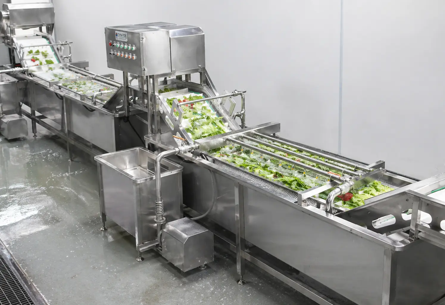


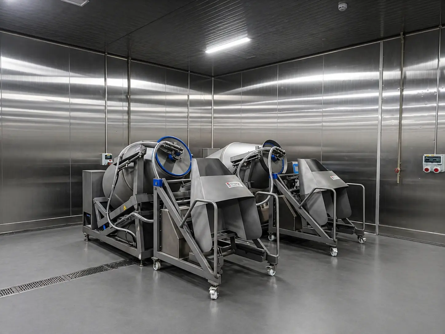


Summary
Leafy vegetable line capacity matching means designing cutting, washing, draining or dewatering, conveying, inspection and packing stages around the same required saleable output—not simply selecting machines with similar catalogue kg/h figures. A line that appears to contain a 1,000 kg/h cutter, a 1,000 kg/h washer and a 1,000 kg/h dewaterer can still fail to produce 1,000 kg of finished product per hour because each number may describe a different material condition, test product, operating mode or time basis.
A decision-grade calculation works backwards from finished saleable kilograms. It accounts for raw-material yield, trimming and cutting losses, batch versus continuous operation, wash residence or contact conditions, product loading, drainage, complete dewatering cycles, changeovers, sanitation, planned and unplanned downtime, buffer capacity and the peak SKU mix. The objective is not to make every machine equally large. It is to create a process in which the required product flow can move through each stage without routinely starving downstream equipment, flooding upstream equipment, shortening a required process step or accumulating excessive work-in-process.
For delicate leafy vegetables, this distinction matters because higher feed rate can change more than productivity. Cut size, product loading and processing conditions can also change wash-water organic load, while insufficient drainage or mismatched batch dewatering can become the practical constraint even when upstream equipment still has unused motor capacity.
Why Leafy-Vegetable Lines That Look Balanced on Paper Still Miss Their Output
Consider a typical fresh-cut operation. Whole lettuce or another leafy raw material is inspected and trimmed, fed into a cutter, washed, transferred to a drainage stage, dewatered and delivered toward inspection, mixing or packing. The cutter runs continuously. The washer also looks continuous. The centrifuge or basket dewaterer works in batches. Production wants a fixed number of finished kilograms before dispatch.
The simplest purchasing approach is to compare the capacity figures of the three major machines. That approach misses the way the process actually behaves.
A cutter may be rated according to kilograms entering the cutting chamber. The washing specification may refer to kilograms of a particular vegetable under a particular feed condition. A batch dewaterer may quote batch load rather than finished kilograms per hour. Product loses mass during trimming, may lose fragments during cutting and washing, temporarily gains surface water after washing, and loses that free water again during dewatering. Meanwhile, the operating day also loses minutes to product changes, sanitation, inspections, adjustments, minor stops and maintenance.
The result is a measurement problem before it is an equipment problem.
If all three machines are compared using different definitions of “capacity,” matching the printed values gives false precision. A better line balance assigns every stage a defined input basis, output basis, cycle basis and operating condition.
Leafy Vegetable Line Capacity Matching Starts with Saleable Output
The most useful starting point is usually not raw input capacity. It is the amount of finished, saleable product that must leave the relevant process section within the available production window.
Suppose a processor must produce a defined quantity of washed and dewatered leafy vegetables for packing during one shift. The line should be calculated backwards from that output. Raw intake is then a consequence of the required finished output and actual process yield.
Separate raw input from saleable output
A basic overall relationship is:
Required raw input = Required saleable output ÷ Overall saleable yield
If 1,000 kg enters receiving but only 820 kg becomes acceptable finished product, the operation does not have a 1,000 kg/h finished-product line merely because receiving can supply 1,000 kg/h.
The more useful calculation separates the yields by process stage:
Overall yield = Trimming yield × Cutting recovery × Washing recovery × Dewatering/handling recovery × any other relevant recovery factor
These factors should come from plant records or product trials. They should not be copied from another processor because cultivar, incoming condition, specifications, cut geometry, rejection criteria and handling practice can change the result materially.
Use the correct capacity requirement at every stage
If the final requirement is 600 kg/h of saleable product, the washer may need to accept more than 600 kg/h before downstream losses. The cutter may need to process still more. Raw trimming may require an even higher incoming rate.
This backward calculation is one of the most important distinctions between equipment capacity and line capacity.
| Process point | Capacity basis to record | Typical planning mistake | What should be verified |
|---|---|---|---|
| Raw receiving / trimming | Raw kg entering per hour | Assuming all incoming mass becomes processable product | Raw condition, reject rate, trim yield, seasonal variation |
| Cutting | Trimmed kg entering cutter and acceptable cut kg leaving | Using cutter nameplate rate as finished-line capacity | SKU, cut size, blade condition, feed continuity, acceptable cut quality |
| Washing | Cut product kg entering under defined wash conditions | Increasing feed until the conveyor is physically full | Residence/contact conditions, product loading, water-management limits and wash performance |
| Drainage | Wet washed product flow | Treating drainage as a zero-time transfer step | Drain time, water carryover, conveyor loading and downstream accumulation |
| Batch dewatering | Usable batch mass divided by complete cycle time | Calculating from spinning time only | Loading, process time, deceleration, unloading, reset and transfer |
| Continuous dewatering | Verified feed rate under target product condition | Increasing speed or feed while ignoring required product condition | Residence, final water carryover, leaf condition and discharge stability |
| Packing / downstream | Saleable finished kg per available hour | Ignoring packing pauses and SKU changes | Pack format, target weights, staffing and changeover frequency |
Convert the Production Schedule into a Required Running Rate
An eight-hour shift does not necessarily provide eight hours of production. If the output target is divided by scheduled hours rather than actual available operating hours, every subsequent equipment calculation is understated.
Start with:
Net planned production minutes = Scheduled minutes − planned sanitation − planned changeover − planned maintenance − other planned line-stopping time
If historical records show that the process also experiences unplanned availability losses, apply the operation’s own measured availability:
Effective production minutes = Net planned production minutes × measured operating availability
Then:
Required saleable running rate = Shift saleable target ÷ effective production hours
This is deliberately different from applying a generic “80% efficiency” or “85% utilization” factor. There is no universal efficiency factor that is automatically correct for a leafy vegetable plant. A line with long, infrequent production runs may behave differently from one producing ten small SKUs each day. A new operation without reliable history should build trial scenarios rather than disguise uncertainty behind an arbitrary percentage.
The same discipline should be applied to labor-dependent preparation. If trimming, sorting or manual feeding constrains the cutter, machine capacity is irrelevant until enough consistently prepared product reaches it.
A useful supporting metric is:
Labor-hours per 1,000 kg saleable product = Direct line labor-hours ÷ saleable kilograms × 1,000
This does not determine whether automation is justified by itself, but it shows where recruitment, training, absenteeism or highly variable manual work may be affecting the line balance.
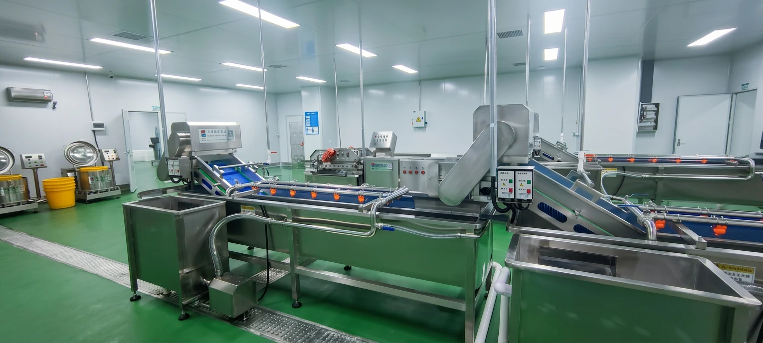
Do Not Match Continuous Machines to Batch Machines by Catalogue kg/h
Cutters and many washing systems operate as continuous-flow equipment. Many dewatering systems operate in discrete batches. Connecting the two creates a scheduling problem.
Continuous-equipment calculation
For a continuous machine, the relevant figure is its verified sustainable feed rate for the intended product and process condition.
The word sustainable matters. If a cutter can momentarily accept a high feed rate but operators must repeatedly stop feeding to clear the outlet, that peak rate is not a useful line-design figure. The same applies to a washer that can physically transport more product only by creating excessive loading or reducing the intended treatment conditions.
Batch-equipment calculation
For one batch dewaterer:
Arithmetic batch capacity = Usable product mass per batch × 60 ÷ complete cycle minutes
The complete cycle begins when the equipment becomes committed to one batch and ends when it is genuinely ready for the next one. Depending on the system, that may include loading, settling or balancing, the programmed dewatering phase, deceleration, unloading, transfer and reset.
If two identical batch units can be operated independently:
Combined arithmetic capacity = capacity per unit × number of simultaneously available units
Even this is not automatically the sustainable line capacity. Shared operators, shared conveyors, transfer devices or a common discharge point can prevent both units from achieving their arithmetic cycle rate.
Why “spin time” is a dangerous denominator
A three-minute dewatering recipe does not create a three-minute batch cycle if loading and discharge require another three minutes. In that example, calculating hourly output from the processing phase alone would overstate potential throughput by roughly a factor of two.
The correct field test is simple: time repeated complete cycles during normal operation, with normal operators and transfer conditions, then measure the actual kilograms handled.
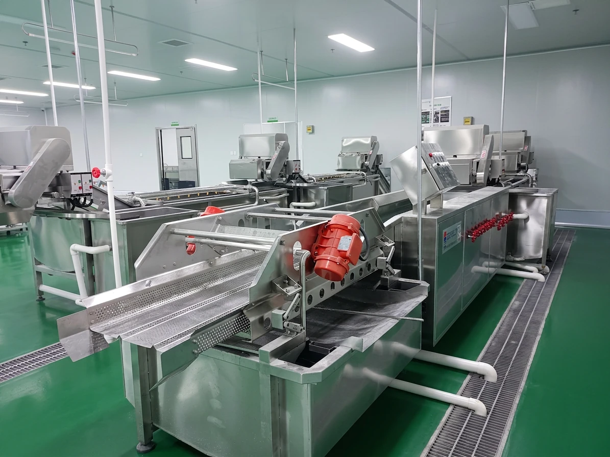
Washing Capacity Is Also a Process-Control Constraint
Washing is where capacity calculations most easily become disconnected from process requirements. A conveyor or flume may continue transporting product as its feed rate increases, but that does not prove the process remains equivalent.
FDA’s 2026 guidance for RTE fresh-cut produce discusses wash-water control specifically because contaminated produce can transfer microorganisms to previously uncontaminated produce through shared wash water. Its examples also recognize feed rate and cut size as variables that can influence the accumulation of organic load in a wash system.
Peer-reviewed work involving romaine lettuce, iceberg lettuce and carrot similarly found that wash-water properties changed with commodity, product loading and cutting conditions; increasing product-to-water ratio and decreasing cut size affected several measures associated with organic loading and chlorine demand.
That makes line balancing more than a mechanical kg/h exercise.
Capacity must preserve the intended wash conditions
For the washer, verify at minimum:
- the commodity and cut geometry being processed;
- feed rate and loading density;
- required product residence or contact conditions;
- water flow and recirculation arrangement;
- applicable wash-water chemistry and monitoring parameters where used;
- temperature conditions;
- organic-load behavior over the intended production run;
- water replacement, filtration or treatment strategy;
- product damage and acceptable physical quality;
- drainage condition at discharge.
A useful residence-time relationship for engineering checks is:
Average product mass in a process zone = Product mass flow per minute × average residence time
If 10 kg/min must remain within a defined process zone for an average of two minutes, roughly 20 kg of product is present in that zone at steady state. Whether the equipment can accommodate that loading without excessive compaction, floating, overlap or uneven treatment must then be verified physically.
Residence time should not be shortened merely to make the washer’s calculated kg/h equal the cutter’s output. If the wash process or a preventive control has defined operating conditions, line capacity must be designed around those conditions rather than the reverse.
A USDA Agricultural Research Service commercial study comparing a single-pass spray system with a conventional flume system for fresh-cut lettuce and cabbage also illustrates why washing technology should be evaluated under defined conditions rather than reduced to one capacity number. Under the tested conditions, wash-water organic load was better controlled in the single-pass system while product microbial levels were similar and sensory quality was equal or better. The study does not establish that one washing architecture is universally superior; it shows that water-management behavior can differ materially between process designs.
Drainage and Dewatering Must Be Treated as Separate Capacity Steps
Processors often talk about “washing and dewatering” as if the product moves directly from one machine to the next. In reality, there is usually a wet transfer condition between them, and that condition matters.
Codex guidance for RTE fresh pre-cut fruits and vegetables states that, except for products packed in liquid, produce should be dried or drained after washing. From a line-balancing perspective, that requirement creates another time and material-state boundary.
A leaf leaving the washer may carry substantial free surface water. That means the instantaneous mass reaching a dewatering unit can include water that is not part of the final saleable vegetable mass. Comparing a wet conveyor-scale reading directly with a finished-product target can therefore mislead the capacity calculation.
Define which basis is being measured:
- vegetable solids/product mass before washing;
- total wet mass immediately after washing;
- drained product mass before active dewatering;
- saleable dewatered product mass.
Where final moisture or surface-water condition is commercially important, it should be incorporated as an acceptance specification rather than assuming that “more centrifugal force” or “longer dewatering” is always better. Delicate leaves can impose a different operating envelope from structurally stronger products.
This is also why a dewatering machine’s throughput should be verified with the real target product. The process recipe, usable batch load and cycle time may vary by SKU.
Calculate WIP and Buffer Capacity Instead of Adding Random Conveyor Length
When a continuous upstream process feeds a batch downstream process, some accumulation is unavoidable. The engineering question is not whether WIP exists, but how much is needed and how much is acceptable.
The basic buffer relationship can be expressed as:
Required buffer ≥ maximum cumulative difference between upstream inflow and downstream outflow during the operating cycle
In mathematical terms, the buffer must absorb the largest positive value of the accumulated flow difference over time.
For example, a continuous washer may discharge steadily while a batch dewaterer accepts product only during loading windows. Product accumulates while the dewaterer is processing, then the buffer level drops during transfer into the next batch.
Adding a larger buffer can make the mechanical line easier to operate, but more WIP is not automatically better. Large queues increase residence time between process steps, occupy floor space, complicate batch identification and can make sanitation or temperature control more difficult. FDA guidance emphasizes time/temperature management for fresh-cut produce, while Codex recommends maintaining RTE pre-cut produce under appropriate cold conditions from cutting onward.
The buffer therefore has two limits:
- minimum operational buffer: enough to decouple normal timing differences and short disturbances;
- maximum acceptable WIP: limited by product quality, time/temperature requirements, traceability, space and hygienic process design.
The goal is controlled surge capacity, not a storage area in the middle of the processing line.
Build the Capacity Model Around the Peak SKU Mix, Not the Average Vegetable
A plant producing only one stable specification has a comparatively straightforward capacity problem. A central kitchen, fresh-cut processor or foodservice supplier producing several leafy SKUs has a scheduling problem as well.
Romaine strips, shredded cabbage, whole leaves, mixed salad components, herbs and other leafy products can impose different loads on cutting, washing, drainage and dewatering. Raw condition can also change by supplier, season or field condition.
A single annual average therefore conceals the conditions most likely to create a bottleneck.
Create an SKU capacity matrix
For each commercially important SKU, record:
- daily and peak-day saleable demand;
- campaign or batch size;
- raw-to-saleable yield;
- trim requirement;
- cut format and cut size;
- verified cutter throughput;
- wash configuration and required operating conditions;
- dewatering usable batch mass or continuous rate;
- complete dewatering cycle;
- changeover time from the preceding SKU;
- sanitation requirements;
- packing format and downstream rate.
From this matrix, examine several scenarios rather than one nominal case:
- the highest-volume SKU;
- the SKU with the slowest cutting or manual preparation;
- the SKU that creates the most demanding washing condition;
- the SKU with the longest dewatering cycle or smallest practical batch;
- the production day with the most changeovers;
- a realistic high-demand mixed-SKU schedule.
Avoid combining every worst-case value into a scenario that could never occur operationally. The purpose is to model credible peak production, not manufacture an artificially impossible design case.
Worked Illustrative Calculation: Matching Cutting, Washing and Batch Dewatering
The following is a hypothetical illustrative calculation. The numbers are not TEEMYEAH machine ratings, customer results or recommended design factors. They exist only to demonstrate the method.
Step 1: Define the shift target and available production time
Assume a processor needs:
- 3,000 kg saleable product per shift;
- an 8-hour scheduled shift = 480 minutes;
- 60 minutes scheduled sanitation;
- 40 minutes total SKU changeover;
- 20 minutes planned inspection or line-stopping checks;
- 92% operating availability during the remaining planned production period, based on this hypothetical plant’s own historical record.
Net planned production time:
480 − 60 − 40 − 20 = 360 minutes
Effective production time:
360 × 0.92 = 331.2 minutes = 5.52 hours
Required saleable running rate:
3,000 ÷ 5.52 = approximately 543 kg/h
Step 2: Work backwards through stage yields
Assume the hypothetical trial data for this SKU show:
- dewatering/handling recovery: 98%;
- washing product recovery: 99%;
- cutting recovery: 97%;
- trimming yield: 90%.
| Flow point | Calculation | Required rate |
|---|---|---|
| Saleable dewatered product | Shift target ÷ effective hours | 543 kg/h |
| Washed product required before dewatering | 543 ÷ 0.98 | Approximately 555 kg/h |
| Acceptable cut product required before washing | 555 ÷ 0.99 | Approximately 560 kg/h |
| Trimmed product required into cutting | 560 ÷ 0.97 | Approximately 577 kg/h |
| Raw material required before trimming | 577 ÷ 0.90 | Approximately 642 kg/h |
The line therefore needs to receive approximately 642 kg/h of this hypothetical raw material while delivering about 543 kg/h saleable output. Designing every machine around “543 kg/h” would understate the requirements of the upstream stages.
Step 3: Compare verified sustainable process rates
Suppose trials indicate that, for this SKU and specification:
- the cutting stage sustainably accepts 700 kg/h of trimmed input while maintaining acceptable cutting quality;
- the washing stage sustainably accepts 650 kg/h of cut product while maintaining the specified process conditions;
- each batch dewaterer accepts a usable 32 kg product load with a complete six-minute cycle.
The cutter exceeds the required 577 kg/h input. The washer exceeds the required 560 kg/h input.
One dewaterer produces an arithmetic batch rate of:
32 × 60 ÷ 6 = 320 kg/h
One unit is clearly insufficient.
Two independent units produce:
320 × 2 = 640 kg/h arithmetic capacity
That appears adequate for the approximately 555 kg/h entering dewatering, subject to verification of transfer, loading, operator interaction and repeated real cycles.
Step 4: Test the peak SKU, not only the first SKU
Now suppose another high-demand SKU uses the same 32 kg usable load but requires a seven-minute complete cycle under its validated quality specification.
Two units would then provide:
32 × 60 ÷ 7 × 2 = approximately 549 kg/h
That is below the approximately 555 kg/h required in the example.
The line that looked comfortably balanced for the six-minute recipe becomes dewatering-limited for the seven-minute recipe. The design team now has meaningful options to evaluate: alter the production schedule, increase dewatering resources, test whether a different validated process can meet the product specification, reduce the required peak rate by extending production time, or introduce another configuration.
What it should not do is shorten the dewatering recipe solely to make the spreadsheet balance.
Use a Capacity Coverage Ratio to Expose Fragile Stages
A simple comparison tool is:
Stage capacity coverage ratio = Verified sustainable stage capacity ÷ required stage input rate
A ratio below 1.00 means the stage cannot meet the calculated requirement under the stated assumptions. A ratio above 1.00 does not automatically make the design safe.
A stage operating only slightly above the calculated requirement may still be fragile if raw-material variability is large, changeovers are unpredictable, the equipment is difficult to recover after a stop, or there is no redundancy. Conversely, oversizing every machine by a large arbitrary percentage can increase capital cost, footprint, water demand, WIP and control complexity without improving finished throughput.
There is no universal “correct” capacity margin. The margin should be justified using actual process variability and the consequence of that stage becoming unavailable.
How to Identify the Real Bottleneck Without Repeating a Generic Bottleneck Study
For this specific line-balancing task, the bottleneck is the stage that prevents the required saleable flow from being maintained under the defined SKU and schedule—not necessarily the machine with the lowest catalogue capacity.
Use a time-based observation sheet and record, for each stage:
- product entering and leaving;
- running, starved, blocked and stopped minutes;
- reason for every material stop;
- batch start and finish times;
- buffer level;
- changeover start and finish;
- operator intervention;
- product rejection or rework;
- water or process-control conditions relevant to the washer.
A cutter that frequently waits for trimmed product is not proven to be undersized. A washer that stops because the downstream batch dewaterer has no empty receiving capacity may not be the bottleneck either. Conversely, a dewatering area that appears busy all day can still be inefficient if much of its cycle is waiting for manual transfer.
The distinction is between machine utilization and constraint utilization. High utilization can be desirable at the true constraint, but forcing every machine to operate continuously often creates unnecessary WIP.
Compare Manual, Semi-Automatic and Integrated Configurations by Flow Behavior
| Configuration | When it can be appropriate | Main capacity advantage | Main capacity risk |
|---|---|---|---|
| Manual / stand-alone machines | Low or irregular volume, many experimental SKUs, frequent recipe changes, limited capital commitment | High scheduling flexibility and easy separation of processes | Manual transfer, feeding and staffing variation can dominate actual throughput |
| Semi-automatic line | Stable core products but significant SKU variability or batch operations | Automates repetitive transfers while retaining buffers and operational flexibility | Poorly designed handoff points can create hidden queues or additional labor |
| More integrated continuous line | Stable recurring demand, defined products, sufficient production hours and validated process conditions | More controlled product flow and less dependence on repeated manual transfers | A disturbance can propagate quickly through connected stages; sanitation and changeover design become more critical |
| Parallel / hybrid configuration | Multiple SKUs with different process requirements or a batch stage constraining an otherwise continuous line | Allows different recipes or parallel capacity at selected constraints | Requires stronger scheduling, routing and traceability discipline |
This comparison explains why more automation is not always the answer to a capacity mismatch. A processor handling small, highly variable orders may gain more from better scheduling, staged equipment and controlled buffers than from physically linking every machine.
Likewise, an operation with stable high-volume demand may find that repeated manual loading between high-throughput machines is itself the dominant constraint.
RTE and RTC Capacity Planning Should Not Be Treated as Identical
The mechanical mathematics may look similar for ready-to-eat and ready-to-cook vegetables, but the food-safety context is not identical.
FDA’s fresh-cut guidance addresses RTE fresh-cut produce as food that can be consumed without a later process expected to significantly minimize biological hazards. Codex guidance for fresh leafy vegetables intended for consumption without cooking likewise emphasizes that there may be no subsequent microbiocidal treatment.
For RTE applications, increasing throughput must therefore be evaluated alongside wash-water control, hygienic zoning, time/temperature management, sanitation and cross-contamination prevention. A mechanical upgrade that doubles upstream feed while overwhelming the validated wash-water control strategy is not a successful capacity upgrade.
RTC products may later receive cooking, but that should not be used as a substitute for appropriate hygiene, process control or applicable regulatory requirements in the preparation facility.
Projects serving both RTE and RTC production should also examine routing. Shared raw receiving may be practical, while downstream process separation, sanitation sequencing, personnel movement, drainage, utensils and product flow may require different controls according to the facility’s hazard analysis.
For a broader discussion of line architecture, see TEEMYEAH’s leafy vegetable processing line solution and the separate RTE salad processing line framework.
Sanitation and Changeover Time Belong in the Capacity Model
Sanitation is frequently excluded from equipment comparisons because it does not happen while product is moving. From a production-capacity perspective, that is precisely why it must be included.
If a machine can process 1,000 kg/h but requires substantially more cleaning time than another configuration, the shift-level output may differ even if their instantaneous processing rates are identical.
FDA’s 2026 guidance addresses hygienic equipment design and recommends considering cleanability when selecting and installing equipment. It discusses smooth and drainable surfaces, access to food-contact surfaces and the ability to remove components for cleaning and maintenance. Those characteristics affect more than food safety; they also influence the minutes available for production.
Track sanitation using real timestamps:
- last acceptable product out;
- equipment access/disassembly complete;
- soil removal complete;
- cleaning complete;
- sanitizing step complete where applicable;
- inspection or verification complete;
- reassembly complete;
- line released for production;
- first acceptable next-SKU product out.
This distinguishes actual sanitation duration from the narrower machine wash-down period.
For multi-SKU facilities, product sequencing can therefore be a capacity decision. Reducing unnecessary changeovers may create more saleable output without changing any major machine.
Capacity Matching Must Include Reliability and Recovery from Stops
Two lines with the same average throughput can behave very differently after a disturbance.
Imagine a batch dewaterer stops for 15 minutes. If the washer continues running, where does its output go? How many kilograms can the buffer hold? Can the washer slow down without losing its required process conditions? Must the cutter stop immediately? Once the dewaterer restarts, does it have enough excess capacity to clear accumulated WIP before the next scheduled changeover?
These questions reveal whether the design has recovery capacity.
Record mean stop duration and actual recovery behavior for important stages. A machine with a high hourly maximum but almost no excess rate above normal demand may take hours to recover from a short interruption.
Redundancy is especially relevant to batch equipment. Two smaller independent dewatering units, for example, behave differently from one larger single processing point during maintenance, although the correct configuration depends on space, labor, cleaning, transfer design, capital cost and target SKUs.
Spare-parts strategy and maintenance access also affect sustainable capacity. A production model based on every critical machine being available 100% of scheduled time is not a line-balance model; it is an assumption.
Do Not Let Automation Create a Faster Route to a Larger Problem
Automation can reduce repetitive handling and stabilize material movement, but it can introduce new process risks.
A tightly coupled line can move an upstream problem into a large quantity of downstream product before operators react. High feed rates can increase buffer pressure. More conveyors and transfer points create more food-contact surfaces to clean. Automated routing can make traceability more complex if batch boundaries are poorly designed. Faster upstream equipment can also overload wastewater, drainage, inspection or packaging systems that were never included in the original equipment comparison.
For delicate vegetables, the consequences are not limited to kilograms per hour. Excessive loading or aggressive transfer can affect leaf condition. Cutting performance depends on blade condition and product feeding, while Codex guidance specifically notes the importance of maintaining cutting edges for product quality and safety.
Equipment cannot replace process design, a food-safety plan, trained personnel or production management.
When Full Line Automation Is Not the Right Capacity Solution
A more integrated line may not be commercially justified when:
- daily volume is low enough that sanitation and changeover dominate the operating schedule;
- the product portfolio changes constantly and recipes have not stabilized;
- raw-material condition is so variable that manual sorting and trimming remain the true process constraint;
- orders arrive in small campaigns that require frequent routing changes;
- the building cannot support hygienic product flow, drainage, access and maintenance around the proposed equipment;
- downstream packing remains far below the proposed processing-line rate;
- the processor has not established real yield, cycle-time or throughput data;
- a proposed automation step would create excessive WIP or eliminate useful process flexibility.
In these situations, phased automation may be the stronger engineering decision. The plant can improve the stage with the clearest verified constraint, measure the new line behavior and decide whether the next investment remains necessary.
Standalone equipment can also be rational where different products require genuinely different routes. Physical integration should follow the process requirement; it should not become the requirement.
Evaluate ROI from Verified Line Output, Not Nameplate Capacity
Once the line balance is technically credible, financial evaluation becomes more meaningful.
Potential benefits may include increased saleable throughput, reduced direct handling labor, fewer overtime hours, more production within the current building or the ability to support new contracts. Potential costs include equipment, utilities, installation, floor-space changes, additional sanitation, preventive maintenance, spare parts, training and possible downstream upgrades.
A basic payback relationship is:
Simple payback period = Incremental investment ÷ verified annual net cash benefit
The important word is verified. Do not calculate payback using a cutter’s theoretical maximum if the dewatering stage means the facility cannot sell the additional output.
Likewise, labor should not automatically be counted as eliminated because a transfer becomes automated. Operators may move into inspection, sanitation, material supply, changeover, monitoring or packaging roles.
Capacity matching improves ROI analysis because it tells management what additional saleable throughput the whole process can realistically support.
A Practical Line-Balance Worksheet for Equipment Selection
Before requesting a final equipment configuration, build one worksheet with one row per process stage and one column per major SKU.
| Worksheet field | Why it matters |
|---|---|
| Saleable demand per shift/day | Defines the real commercial output requirement |
| Scheduled and effective production minutes | Converts demand into required running rate |
| Raw yield and stage yields | Converts finished output into upstream flow requirements |
| Required input/output rate by stage | Prevents comparison of unlike kg/h figures |
| Continuous or batch operation | Determines the correct capacity calculation |
| Usable batch mass | Defines real batch quantity rather than vessel volume |
| Complete batch cycle | Determines actual batch throughput |
| Residence/contact requirement | Prevents speed increases from changing the intended process |
| Changeover and sanitation | Defines time genuinely available to produce |
| Historical availability | Introduces actual reliability into the model |
| Minimum and maximum WIP | Controls starvation, blocking and excessive accumulation |
| Peak-SKU scenario | Tests the line against credible difficult production days |
For projects still defining equipment, TEEMYEAH’s equipment capacity verification guide can be used to establish how individual equipment figures should be tested. The present article addresses the next question: how those verified machines should be balanced together.
Validate the Line Balance Before Freezing the Configuration
A spreadsheet should narrow the solution. Product testing should confirm it.
A useful validation plan includes representative raw material and, where practical, the SKUs expected to be most demanding. Measure the actual process rather than asking only whether each machine runs.
- Confirm incoming condition. Record commodity, supplier or source where relevant, raw temperature, trim condition and abnormal soil or damage.
- Measure raw and saleable mass. Establish the mass balance through trimming, cutting, washing and dewatering.
- Verify cutting. Record sustainable feed, accepted cut quality, reject or fragment generation and blade setup.
- Verify washing under intended conditions. Record product feed, loading, process time or residence, water-management parameters and discharge condition.
- Measure drainage. Determine how much wet product reaches dewatering and whether transfer becomes unstable.
- Time complete dewatering cycles. Include loading through readiness for the next batch.
- Observe the interface. Record starvation, blocking, buffer level and operator waiting.
- Repeat. A single successful short run does not demonstrate sustainable throughput.
- Test changeover. Measure the real transition between commercially important SKUs.
- Recalculate the line. Replace preliminary assumptions with measured values before final configuration.
If the dewatering calculation indicates that batch handling is likely to be the limiting stage, an automated system such as the TW-980LB vegetable dehydration line can be evaluated as a configuration option without assuming in advance that it is the correct answer. Similarly, a cutter such as the TW-801P multifunctional vegetable cutter should be assessed against the intended SKU, cut specification and required upstream rate rather than selected from a generic capacity figure alone.
Conclusion: Match the Process, Not the Machine Labels
A properly matched leafy vegetable line does not require every machine to display the same kg/h figure. It requires every process step to support the same commercial output objective under its own real operating constraints.
Begin with saleable output and effective production time. Work backwards through yield to calculate the mass that each upstream stage must handle. Separate continuous rates from batch-cycle capacity. Protect washing residence and process-control requirements. Include drainage and complete dewatering cycles. Model changeovers, sanitation and downtime. Size WIP buffers according to flow variation but limit accumulation according to product, temperature, hygienic and traceability requirements. Most importantly, repeat the calculation for the peak SKU mix rather than relying on an average product.
The result is more than equipment selection. It is a process-flow design that connects raw-material behavior, production scheduling, hygienic operation, machinery and finished demand. That is the level at which capacity should be matched before an integrated vegetable processing line is finalized.
Calculate Your Matched Line Capacity
If you are planning a new leafy vegetable processing line or upgrading an existing cutting, washing and dewatering section, prepare the raw materials, finished products, target saleable capacity, working hours, SKU mix, cut specifications, current cycle times and available layout.
TEEMYEAH can use those inputs to discuss a preliminary process flow, equipment configuration, capacity balance and layout concept for a central kitchen, fresh-cut vegetable facility, RTC operation or RTE production project. Where the product behavior is uncertain, representative product testing can be used to replace assumed throughput with measured process data before the configuration is finalized.
For the broader application framework, review the fresh-cut vegetable processing solution, then use the line-balance worksheet above to define the capacity information required for a project discussion.
FAQ
1. What is leafy vegetable line capacity matching?
Leafy vegetable line capacity matching is the process of calculating how much product each cutting, washing, drainage, dewatering and downstream stage must handle to achieve a defined saleable output. The calculation should use the actual material state at each stage rather than comparing catalogue kg/h values directly. It also includes effective production time, process yield, continuous versus batch operation, wash residence or control conditions, complete dewatering cycles, changeovers, sanitation, downtime and WIP. A matched line is therefore one in which the required flow can pass through the process sustainably without routinely starving, blocking or overloading another stage.
2. Should the cutter, washer and dewaterer all have the same rated kg/h?
No. Equal rated capacities do not necessarily create a balanced line because the machines may measure different product states and operate differently. A cutter may be rated by trimmed input, a washer by cut-product feed, while a dewaterer may be specified by batch mass. Yield losses also mean upstream stages usually handle more vegetable mass than the final saleable output. Match each stage to its required input rate after accounting for yield, operating time and process conditions. The relevant comparison is verified sustainable capacity versus the required rate for that specific stage, not whether three brochure figures happen to be identical.
3. How do I calculate the hourly capacity of a batch vegetable dewaterer?
Use the usable product mass per batch and the complete batch cycle. The basic arithmetic is: usable batch mass × 60 ÷ complete cycle minutes. Complete cycle time should include loading, the dewatering program, deceleration, unloading, transfer and reset until the machine is genuinely ready for the next batch. Do not calculate capacity from spinning time alone. If several units operate in parallel, their arithmetic capacity can be combined only if operators, conveyors and transfer equipment allow them to cycle independently. Repeated production trials should confirm the sustainable result with the intended leafy vegetable and recipe.
4. How much extra capacity should each machine have above the target line rate?
There is no universal percentage that should automatically be added to every machine. The required margin depends on product variability, historical downtime, consequences of a stop, changeover frequency, raw-material condition, availability of parallel equipment and the ability of downstream stages to absorb fluctuations. Calculate a stage capacity coverage ratio by dividing verified sustainable stage capacity by the required stage rate, then test realistic operating scenarios. A ratio barely above 1.00 may be fragile, but extreme oversizing can add unnecessary capital cost, footprint, water demand and WIP. Capacity margin should be justified by measured or credible project-specific variability.
5. Why can washing become the bottleneck even when the washer can physically transport more product?
Because mechanical transport is only one part of washing capacity. Product feed rate, cut size, loading, residence conditions, water management and organic load can influence the behavior of a fresh-cut washing process. FDA guidance specifically recognizes feed rate and cut size as relevant parameters in examples involving wash-water organic load. Increasing conveyor speed or product loading may therefore change the process instead of simply increasing throughput. The usable washing capacity is the rate at which the system can continuously meet the defined product, water-management and food-safety conditions—not the maximum amount that can physically pass through the tank or conveyor.
6. How should WIP be sized between a continuous washer and a batch dewaterer?
Size the buffer from the maximum cumulative difference between upstream inflow and downstream outflow over the batch cycle. Product will accumulate while the dewaterer is unavailable for loading and decrease when the next batch transfers. The buffer must be large enough to prevent routine upstream blocking, but it should not become uncontrolled storage. Set a maximum WIP limit based on acceptable hold time, product quality, time/temperature control, traceability, hygienic design and available space. Simulating several consecutive cycles is more reliable than selecting conveyor or hopper volume simply because extra physical space is available.
7. Should line capacity be calculated from raw kilograms or finished kilograms?
Use both, but do not confuse them. Commercial demand is normally best defined as saleable finished kilograms, while each upstream machine must be sized according to the mass actually entering that stage. Begin with the required finished output, divide by the recovery or yield of each downstream stage, and work backwards toward raw receiving. This creates a stage-by-stage mass balance. If 600 kg/h of finished product requires 700 kg/h entering cutting and still more raw material before trimming, a machine rated for 600 kg/h upstream will not meet the finished-output target even though its number matches the sales requirement.
8. Does a higher-capacity cutter automatically increase total leafy vegetable line output?
No. The cutter increases finished output only when cutting is the active constraint or when additional cutting capacity improves the schedule without overloading later stages. If washing, batch dewatering, manual inspection or packing already limits the line, a faster cutter may simply create more WIP. It can also increase the rate at which organic material enters the wash system if more cut product is produced. Before upgrading cutting capacity, calculate the required flow through every downstream stage and observe where the current line is starved, blocked or stopped. Capacity investment should target the process constraint rather than the machine that is easiest to replace.
9. Is a fully automated line always better for high-volume leafy vegetable processing?
No. Higher, stable recurring demand can make integrated automation attractive, particularly where manual transfers are limiting flow, but automation also increases coupling between process stages. A stop can propagate quickly, and additional conveyors or transfer systems create more surfaces to clean and maintain. Facilities with frequent small batches, highly variable raw materials or many changing recipes may benefit from semi-automatic or hybrid layouts that preserve routing flexibility. The appropriate level of automation should follow the SKU profile, labor requirement, hygienic design, production schedule, available floor space and verified capacity balance rather than a general assumption that maximum integration is always superior.
10. What information should I provide a supplier for accurate leafy vegetable line sizing?
Provide target saleable output, production hours, major SKUs, peak-day mix, raw-material condition, raw-to-saleable yields if known, trim requirements, cut formats, RTE or RTC application, washing requirements, dewatering target, packaging rate, sanitation schedule, changeover frequency and available layout. Existing processors should also provide measured cycle times and actual throughput by stage. Photos, videos or trial samples can help clarify product behavior. A supplier can make a more meaningful configuration when capacity is defined as a process requirement rather than a single statement such as “we need a 1,000 kg/h vegetable line.”
Data and Source Note
This article uses the U.S. Food and Drug Administration’s 2026 Guide to Minimize Biological Hazards in Ready-to-Eat Fresh-Cut Produce for the discussion of fresh-cut RTE biological hazards, wash-water process control, the influence of processing conditions such as feed rate and cut size in FDA’s validation examples, hygienic equipment design, sanitation and time/temperature management. The document is U.S.-focused guidance, contains nonbinding recommendations and should not be interpreted as a universal equipment specification or as a prescribed capacity factor.
FAO/WHO Codex Alimentarius Code of Hygienic Practice for Fresh Fruits and Vegetables, CXC 53-2003, including its annexes concerning RTE fresh pre-cut fruits and vegetables and fresh leafy vegetables, supports the discussion of washing, draining or drying after washing, knife condition, cold handling and the special context of leafy vegetables intended for consumption without a later microbiocidal step. Codex provides international hygienic guidance; regulatory implementation and approval of specific treatments vary by jurisdiction.
The 2018 USDA Agricultural Research Service commercial study by Bornhorst and co-authors, published in Postharvest Biology and Technology, compared single-pass spray and conventional flume washing during commercial fresh-cut lettuce and cabbage processing. Its findings are cited only to demonstrate that wash-system design can change wash-water behavior under defined operating conditions. The study does not establish a universal preferred washing technology or universal commercial capacity.
The supplied 2019 PLOS ONE source resolves to the paper by Li and co-authors, Dynamic changes in the physicochemical properties of fresh-cut produce wash water as impacted by commodity type and processing conditions. It studied romaine lettuce, iceberg lettuce and carrot under controlled wash-water experiments and showed that commodity, loading and cutting conditions influence wash-water properties. It provides process-science evidence, not production-line capacity ratings.
López-Gálvez and co-authors’ 2019 Food Microbiology study compared testing of centrifuge effluent water with finished fresh-cut lettuce for detection of an E. coli indicator. Although results from the two matrices frequently coincided, the authors concluded that the centrifuge-water alternative was not reliable because of low sensitivity. It is therefore relevant here as evidence that a convenient downstream sampling point should not automatically be treated as a substitute for an established microbiological sampling or food-safety verification program.

